Other operations

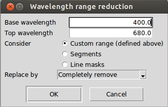
Wavelength range reduction

The current active spectrum can be cut by selecting "Operations - Wavelength range reduction" and specifying a base and top wavelength or using directly the defined segments/line regions. The user can also choose to replace the removed fluxed by zeros.

Apply mathematical expression

The wavelength, fluxes and error values of the active spectrum can be modified by applying a mathematical expression which can contain any combination of the following functions:

• sin(x) Trigonometric sine, element-wise.
• cos(x) Cosine elementwise.
• tan(x) Compute tangent element-wise.
• arcsin(x) Inverse sine, element-wise.
• arccos(x) Trigonometric inverse cosine, element-wise.
• arctan(x) Trigonometric inverse tangent, element-wise.
• arctan2(x1, x2) Element-wise arc tangent of x1/x2 choosing the quadrant correctly
• sinh(x) Hyperbolic sine, element-wise.
• cosh(x) Hyperbolic cosine, element-wise.
• tanh(x) Compute hyperbolic tangent element-wise.
• arcsinh(x) Inverse hyperbolic sine elementwise.
• arccosh(x) Inverse hyperbolic cosine, elementwise.
• arctanh(x) Inverse hyperbolic tangent elementwise.
• around(a[, decimals, out]) Evenly round to the given number of decimals.
• floor(x) Return the floor of the input, element-wise.
• ceil(x) Return the ceiling of the input, element-wise.
• exp(x) Calculate the exponential of all elements in the input array.
• log(x) Natural logarithm, element-wise.
• log10(x) Return the base 10 logarithm of the input array, element-wise.
• log2(x) Base-2 logarithm of x.
• sqrt(x) Return the positive square-root of an array, element-wise.
• absolute(x) Compute the absolute values elementwise.
• add(x1, x2) Add arguments element-wise.
• multiply(x1, x2) Multiply arguments element-wise.
• divide(x1, x2) Divide arguments element-wise.
• power(x1, x2) First array elements raised to powers from second array, element-wise.
• subtract(x1, x2) Subtract arguments, element-wise.
• mod(x1, x2) Return element-wise remainder of division.

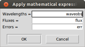
The functionality can be found in "Operations - Apply mathematical expression" and the current values can be used as variable names "waveobs", "flux" and "err". Some examples of the utility of this functionality:

• Convert the wavelengths from Angstroms to nanometers by dividing the wavelengths by 10: Waves = waveobs / 10
• Change the scale of the fluxes: Fluxes = power(flux, 2)
• Modify the errors by using a percentage relative to the flux: Errors = flux * 0.05
• Assign a constant value to the error values: Errors = err * 0.0 + 1.0

The result of the mathematical operation should always be an array with the same number of elements as the original spectrum.

Fluxes and errors cleaning

In order to filter bad measurements out, the current active spectrum can be cleaned by selecting "Operations - Clean fluxes and errors". The user has to specify a base and top flux and error.

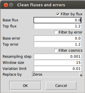
Additionally, the cleaning can be done by considering the mean and standard deviation of a limited region (between a top and base flux level). This option can be useful to remove cosmics residuals although it should be used carefully since it would remove also emission lines.

Finally, the user can chose to completely remove the fluxes or replace them by the continuum instead of zeros.

Clean telluric regions

Through the menu "Operations - Clean telluric regions", one can clean the regions of the spectrum that may be affected by telluric lines. For that purpose it is needed: the radial velocity of the spectrum (it is recommended to be radial velocity corrected, so the radial velocity would be zero), the minimum depth of the telluric lines to consider and the region around those lines to be cleaned (in km/s). The user can chose to completely remove the fluxes or replace them by the continuum instead of zeros.

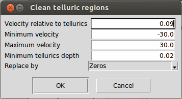
By default a margin of +/-30 km/s is suggested, since it represents the typical maximum velocity ranges where the telluric lines may be. For instance, considering a fictitious star that has zero radial velocity respect to the sun, when it is observed from earth a radial velocity might be measured due to the rotation of the earth around the sun. This radial velocity respect to the each will typically be between -30 and +30 km/s for this fictitious star depending on the region of the sky that it is observed.

This functionality is mainly useful when the spectrum is going to be used as a template for measuring the radial velocity of another spectrum. Cleaning all this fluxes from the template reduces the impact of potential telluric lines in the spectrum to be measured.

Spectrum re-sampling

By selecting "Operations - Resample spectrum", the current active spectrum can be uniformly re-sampled within a wavelength range and with a fixed step.

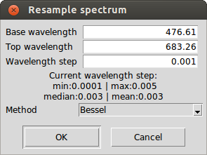
The interpolation method can be linear, bessel (4 points are considered at each interpolated point, the result tends to be smoother than the linear interpolation but it is not recommended) or spline (it might help to smooth the spectrum, but again, not generally recommended).

Spectra combination

All the open spectra can be combine through "Edit - Combine all spectra" by using the mean/median, subtracting (active spectrum minus the rest), co-adding or dividing (active spectrum divided by the rest) the flux values. It is recommended that before doing so, all the spectra should be aligned (e.g., radial velocity corrected) and they should have the same resolution.

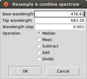
The process does the following operations:

• It builds a common wavelength coordinates which will depend on the ranges and wavelength step specified by the user
• It homogenizes all the spectra by interpolating the flux at each point of the common wavelength coordinates. It is worth noting that the visualized spectra is not replaced by the homogenized version, they are only used internally by the combine function.
• The homogenized spectra is combined and the result is displayed.